October 27, 2026 / Web Development
Projectile motion equations: a worked example for animation
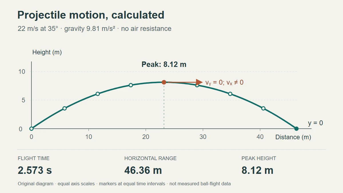
Projectile motion equations let you calculate the position of an ideal object after launch. They are useful for a classroom problem, a trajectory preview or a simple browser animation. The model assumes constant downward gravity and no air resistance; it should not be presented as a measured prediction of every real ball flight.
With horizontal position x, upward-positive height y, and elapsed time t, the working equations are:
x(t) = x₀ + v₀ₓty(t) = y₀ + v₀ᵧt − ½gt²
The starting position is (x₀, y₀). The values v₀ₓ and v₀ᵧ are the initial horizontal and vertical velocities. Gravity is written as a positive magnitude g, so its contribution has a minus sign when up is positive.
Choose the coordinates and units first
If launch speed is v₀ and angle θ is measured above the horizontal, resolve the velocity into components:
v₀ₓ = v₀ cos θv₀ᵧ = v₀ sin θ
Use metres, seconds and metres per second throughout the example below, with g = 9.81 m/s². This is a chosen near-Earth approximation. Changing the length unit means changing the numerical value of gravity too; a value expressed in feet per second squared cannot be used with distances in kilometres or miles without conversion.
The OpenStax treatment of projectile motion sets out the independent horizontal and vertical motions under these assumptions. Equal launch and landing heights are needed for some shortcut formulas, but not for the two position equations.
What happens at the highest point?
The vertical velocity changes with time:
vᵧ(t) = v₀ᵧ − gt
For an upward launch, the peak occurs when that velocity reaches zero, giving t_peak = v₀ᵧ / g. The object still has its horizontal velocity. Zero vertical velocity does not mean that the entire object has stopped.
The two terms v₀ᵧt and ½gt² in the height equation are not equal at the peak. They cancel when the object returns to its launch height. At the peak, the first is twice the second, leaving a positive height above the starting point.
Flight time, peak height and range
For an upward launch that returns to the same height, the nonzero return time and horizontal range are:
| Quantity | Formula | Condition |
|---|---|---|
| Return time | T = 2v₀ᵧ / g |
Landing height equals launch height; initial vertical velocity is positive |
| Peak rise above launch | H = v₀ᵧ² / (2g) |
Upward initial vertical velocity |
| Horizontal range | R = v₀ₓT = v₀² sin(2θ) / g |
Same-height return with the stated gravity-only model |
If the launch height is not zero, the peak’s height in those coordinates is y₀ + H. The rise H is not automatically a height above the ground.
At fixed initial speed, 45° maximizes the same-height range because it maximizes sin(2θ). Complementary angles such as 30° and 60° give equal ranges in this model. Neither result establishes an optimum for a real sports ball with drag, spin or different landing conditions.
Worked example: 22 m/s at 35°
Take an ideal particle launched from x₀ = y₀ = 0 at 22 m/s and 35°. The landing surface is at the launch height. This is a calculation with chosen inputs, not a recorded kick or throw.
- Horizontal velocity:
22 cos 35° ≈ 18.0213 m/s. - Initial vertical velocity:
22 sin 35° ≈ 12.6187 m/s. - Peak time:
12.6187 / 9.81 ≈ 1.2863 s. - Return time:
2 × 12.6187 / 9.81 ≈ 2.5726 s. - Horizontal range: approximately
46.36 m. - Peak rise: approximately
8.12 m.
The accompanying diagram uses equal distance scales on both axes and marks equal time intervals. At its peak the vertical velocity is zero, while horizontal motion continues. Keep full precision during the calculation and round the displayed answers at the end.
Range alone does not tell you whether the particle passes through a target at an earlier distance. For that question, calculate the time at the target’s horizontal position and substitute it into the height equation.
Different landing heights require the vertical equation
Let Δy = y_landing − y₀. Substituting the landing height gives a quadratic:
½gT² − v₀ᵧT + Δy = 0
Its candidate times are:
T = (v₀ᵧ ± √(v₀ᵧ² − 2gΔy)) / g
A negative expression inside the square root means the chosen height is not reached in this ideal model. A height above the launch point can be reached twice, once while rising and once while falling. Both times can be positive, so “take the positive root” is not a complete instruction. Choose the intersection corresponding to the event you are modelling.
For a separate example, give a particle horizontal speed 10 m/s and zero initial vertical velocity, starting 2 m above a horizontal landing surface. Its fall time is √(2 × 2 / 9.81) ≈ 0.6386 s, and it travels approximately 6.39 m horizontally. A zero launch angle therefore does not imply zero range when the landing is lower.
Describing the path without time
If v₀ₓ ≠ 0, eliminate time using t = (x − x₀) / v₀ₓ:
y = y₀ + (v₀ᵧ/v₀ₓ)(x − x₀) − g(x − x₀)²/(2v₀ₓ²)
This gives a parabola for a nonvertical launch in the gravity-only model. For a vertical launch, horizontal position stays constant; use the time equations instead of dividing by zero.
Using the equations in an animation
For a trajectory with no collisions or changing forces, calculate the position directly from elapsed time. The following function returns displacement in metres from the launch point. It assumes valid numerical inputs and a gravity magnitude expressed in metres per second squared.
function projectilePosition(elapsedSeconds, initialSpeed, launchAngleDegrees, gravity = 9.81) {
  const angleRadians = launchAngleDegrees * Math.PI / 180;
  const horizontalVelocity = initialSpeed * Math.cos(angleRadians);
  const verticalVelocity = initialSpeed * Math.sin(angleRadians);

  return {
    horizontalMetres: horizontalVelocity * elapsedSeconds,
    verticalMetres: verticalVelocity * elapsedSeconds
      - 0.5 * gravity * elapsedSeconds ** 2
  };
}
For a downward-positive screen, one possible mapping is screenY = launchScreenY − pixelsPerMetre × verticalMetres. Use the same scale for horizontal displacement if the drawing is meant to preserve physical angles.
The requestAnimationFrame documentation explains that its timestamp is measured in milliseconds. Subtract the initial timestamp and divide by 1000 before passing elapsed time to this function. Do not assume every displayed frame lasts exactly 16.67 milliseconds.
The function draws a point on an unrestricted path. It does not detect a floor, stop at landing, apply a bounce or respond to another force. Add those behaviours explicitly for an interactive scene. If the equations are being taught, keep their assumptions and numerical results available as text alongside the animation.
Where drag changes the model
The NASA drag equation gives the magnitude D = ½ρCᴅAV², using air density, drag coefficient, reference area and speed relative to the air. A force’s direction and its effect on acceleration also matter when adding it to a motion model.
In the gravity-only equations there is no air-force term. Merely adding a constant wind speed to the initial horizontal velocity does not model wind acting on the object during flight. Likewise, a blanket threshold such as “drag below ten percent of gravity guarantees an accurate range” does not specify an error bound for an entire trajectory.
Use the simple model when its assumptions suit the task, and state when they do not. A more detailed simulation needs a defined force model and appropriate numerical or analytical treatment, rather than a cosmetic change to the gravity-only range formula.
Checks before trusting the result
- State whether up or down is positive and keep the gravity sign consistent.
- Check angle units. JavaScript’s trigonometric functions take radians; the example converts degrees explicitly.
- Distinguish a rise above launch from height above the ground.
- Check whether launch and landing heights match before using a shortcut for range or time.
- Verify the starting point, peak velocity and landing point with the same input values.
For the interface around a simulation, the studio’s web accessibility guide offers further reading. Other design and development notes are available in the blog.